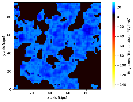
Running and Plotting Coeval Cubes

The aim of this tutorial is to introduce you to how 21cmFAST does the most basic operations: producing single coeval cubes, and visually verifying them. It is a great place to get started with 21cmFAST.

# We change the default level of the logger so that
# we can see what's happening with caching.
import logging

import matplotlib.pyplot as plt

logger = logging.getLogger("py21cmfast")
logger.setLevel(logging.INFO)

from tempfile import mkdtemp

import py21cmfast as p21c

# For plotting the cubes, we use the plotting submodule:
from py21cmfast import plotting

print(f' Using 21cmFAST version {p21c.__version__}')

 Using 21cmFAST version 4.3.dev77+g0d19d34ee

Run a simulation using run_coeval and generate_coeval

Specifying input parameters is a topic covered in a different tutorial. Here, we want something small and fast:

inputs = p21c.InputParameters.from_template(
    ["simple", 'small'], random_seed=1234
)

The simplest (and typically most efficient) way to produce a coeval cube is simply to use the run_coeval method. This consistently performs all steps of the calculation, re-using any data that it can without re-computation or increased memory overhead.

First we make a temporary cache to store our fields, in larger runs 21cmFAST can store its outputs in an OutputCache to avoid unnecessary regeneration

cache = p21c.OutputCache(mkdtemp())

coevals = p21c.run_coeval(
    inputs=inputs,
    out_redshifts=[8, 9, 10],
    cache=cache,
    progressbar=True
)

/home/steven/Documents/work/21cmfast/21cmfast/.claude/worktrees/issue-565-discussion-46670d/.venv/lib/python3.13/si
te-packages/rich/live.py:260: UserWarning: install "ipywidgets" for Jupyter support
  warnings.warn('install "ipywidgets" for Jupyter support')

The generate_coeval method is a generator, which can be called as follows:

coevals = []
for coeval,in_outputs in p21c.generate_coeval(
    inputs=inputs,
    out_redshifts=[8, 9, 10],
    cache=cache,
):
    if in_outputs:
        coevals.append(coeval)

Note that this run was much faster, since we cached the outputs from the previous run, and they were simply loaded instead of re-calculated

There are a number of possible inputs for generate/run_coeval, which you can check out either in the API reference or by calling help(p21c.run_coeval).

Notably, in our case here, the out_redshifts must be given: these are the redshifts at which we compute the coeval boxes. When the simulation requires evolution over cosmic history, coeval boxes will be computed at every node as well as any out_redshifts specified.

Since the function is a generator, it yields a Coeval box on each iteration. These boxes can be saved or post-processed before completing the next iteration, allowing arbitrarily flexible computations to be performed. The second returned values is a boolean which tells you whether you are at a requested output point in out_redshifts.

We’ve also given a cache parameter: this specifies a directory in which the various component calculations of this simulation will be cached. By default, this will occur in the current directory, but here we are using a temporary directory for convenience. While by default all sub-components are written into the cache, this can be turned off altogether, or toggled per subcomponent. The main reason to use the cache is if you might want to re-use simulated component boxes in other simulations in the future. A prime example of this is the InitialConditions, for which a single simulation can be used for a multitude of astrophysical simulations with varying AstroParams.

The output on each iteration is, as we have mentioned, a Coeval object. This is a simple object that contains a number of 3D arrays of data, one for each of the component fields simulated. They can be accessed as attributes of the object:

coevals[0].redshift

10.0

A list of all simulated fields can be accessed:

coevals[0].get_fields()

['lowres_density',
 'lowres_vx',
 'lowres_vy',
 'lowres_vz',
 'hires_density',
 'hires_vx',
 'hires_vy',
 'hires_vz',
 'lowres_vx_2LPT',
 'lowres_vy_2LPT',
 'lowres_vz_2LPT',
 'hires_vx_2LPT',
 'hires_vy_2LPT',
 'hires_vz_2LPT',
 'lowres_vcb',
 'density',
 'velocity_z',
 'velocity_x',
 'velocity_y',
 'neutral_fraction',
 'ionisation_rate_G12',
 'z_reion',
 'mean_free_path',
 'cumulative_recombinations',
 'kinetic_temperature',
 'unnormalised_nion',
 'unnormalised_nion_mini',
 'brightness_temp',
 'tau_21',
 'spin_temperature',
 'xray_ionised_fraction',
 'kinetic_temp_neutral',
 'J_21_LW',
 'count',
 'halo_mass',
 'halo_stars',
 'halo_stars_mini',
 'halo_sfr',
 'halo_sfr_mini',
 'halo_xray',
 'n_ion',
 'whalo_sfr']

The Coeval object also maintains a reference to the input parameters:

coevals[0].inputs

cosmo_params: CosmoParams(_SIGMA_8=None, hlittle=0.6766, OMm=0.30964144154550644, OMb=0.04897468161869667, POWER_INDEX=0.9665, _A_s=None, OMn=0.0, OMk=0.0, OMr=8.6e-05, OMtot=1.0, Y_He=0.24, wl=-1.0)
simulation_options: SimulationOptions(HII_DIM=64, _BOX_LEN=None, _DIM=None, _HIRES_TO_LOWRES_FACTOR=None, _LOWRES_CELL_SIZE_MPC=None, NON_CUBIC_FACTOR=1.0, N_THREADS=1, SAMPLER_MIN_MASS=100000000.0, SAMPLER_BUFFER_FACTOR=2.0, N_COND_INTERP=200, N_PROB_INTERP=400, MIN_LOGPROB=-12.0, HALOMASS_CORRECTION=0.89, PARKINSON_G0=1.0, PARKINSON_y1=0.0, PARKINSON_y2=0.0, Z_HEAT_MAX=35.0, ZPRIME_STEP_FACTOR=1.1, MIN_XE_FOR_FCOLL_IN_TAUX=0.001, INITIAL_REDSHIFT=300.0, DELTA_R_FACTOR=1.1, DENSITY_SMOOTH_RADIUS=0.2, DEXM_OPTIMIZE_MINMASS=100000000000.0, DEXM_R_OVERLAP=2.0, CORR_STAR=0.5, CORR_SFR=0.2, CORR_LX=0.2, K_MAX_FOR_CLASS=None)
matter_options: MatterOptions(HMF='ST', _USE_RELATIVE_VELOCITIES=None, V_CB_MODEL='NONE', POWER_SPECTRUM='EH', PERTURB_ON_HIGH_RES=False, USE_INTERPOLATION_TABLES='hmf-interpolation', MINIMIZE_MEMORY=False, KEEP_3D_VELOCITIES=False, SAMPLE_METHOD='MASS-LIMITED', FILTER='spherical-tophat', HALO_FILTER='spherical-tophat', SMOOTH_EVOLVED_DENSITY_FIELD=False, DEXM_OPTIMIZE=False, PERTURB_ALGORITHM='2LPT', USE_FFTW_WISDOM=False, SOURCE_MODEL='E-INTEGRAL')
astro_params: AstroParams(HII_EFF_FACTOR=30.0, F_STAR10=-1.3, ALPHA_STAR=0.5, F_STAR7_MINI=-2.8, ALPHA_STAR_MINI=0.5, F_ESC10=-1.0, ALPHA_ESC=-0.5, F_ESC7_MINI=-2.0, M_TURN=8.7, R_BUBBLE_MAX=32.0, R_BUBBLE_MIN=0.620350491, ION_Tvir_MIN=4.69897, L_X=40.5, L_X_MINI=40.5, NU_X_THRESH=500.0, X_RAY_SPEC_INDEX=1.0, X_RAY_Tvir_MIN=4.69897, F_H2_SHIELD=0.0, t_STAR=0.5, A_LW=2.0, BETA_LW=0.6, A_VCB=1.0, BETA_VCB=1.8, UPPER_STELLAR_TURNOVER_MASS=11.447, UPPER_STELLAR_TURNOVER_INDEX=-0.6, SIGMA_STAR=0.25, SIGMA_LX=0.5, SIGMA_SFR_LIM=0.19, SIGMA_SFR_INDEX=-0.12, T_RE=20000.0, _FIXED_VAVG=None, V_CB_AVG_DEBUG=27.0, POP2_ION=5000.0, POP3_ION=44021.0, PHOTONCONS_CALIBRATION_END=3.5, CLUMPING_FACTOR=2.0, ALPHA_UVB=5.0, R_MAX_TS=500.0, N_STEP_TS=40, MAX_DVDR=0.2, DELTA_R_HII_FACTOR=1.1, NU_X_BAND_MAX=2000.0, NU_X_MAX=10000.0)
astro_options: AstroOptions(USE_MINI_HALOS=False, USE_X_RAY_HEATING=True, USE_CMB_HEATING=True, USE_LYA_HEATING=True, _INHOMO_RECO=None, USE_TS_FLUCT=False, _FIX_VCB_AVG=None, USE_EXP_FILTER=False, CELL_RECOMB=False, LYA_MULTIPLE_SCATTERING=False, USE_ADIABATIC_FLUCTUATIONS=True, PHOTON_CONS_TYPE='no-photoncons', USE_UPPER_STELLAR_TURNOVER=False, M_MIN_in_Mass=True, HALO_SCALING_RELATIONS_MEDIAN=False, HII_FILTER='sharp-k', HEAT_FILTER='spherical-tophat', IONISE_ENTIRE_SPHERE=False, RECOMB_MODEL='none', INTEGRATION_METHOD_ATOMIC='GAUSS-LEGENDRE', INTEGRATION_METHOD_MINI='GAUSS-LEGENDRE')

We can also save/load a Coeval object to disk:

coevals[0].save(cache.direc / "coeval.h5")

Note that, if you are also using the cache (as we are), then saving the Coeval object creates redundant data on disk. The files created by Coeval are more convenient for saving, sharing and using in further post-processing, but are not easily used for caching purposes.

The file that we wrote can be easily read:

coeval10 = p21c.Coeval.from_file(cache.direc / "coeval.h5")

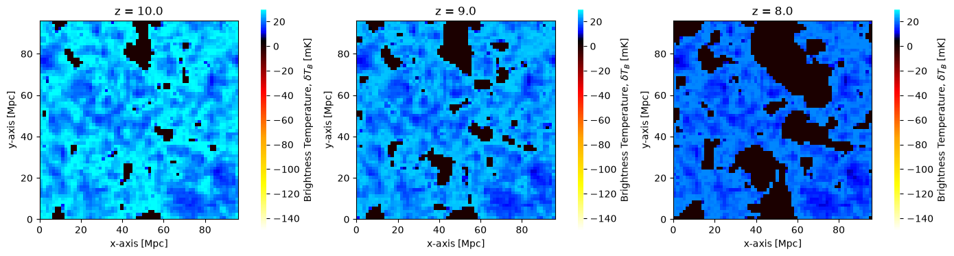
Some convenient plotting functions exist in the plotting module. These can work directly on Coeval objects, or any of the output structs (as we’ll see further on in the tutorial). By default the coeval_sliceplot function will plot the brightness_temp, using the standard traditional colormap:

fig, ax = plt.subplots(1, 3, figsize=(14, 4))
for i, coeval in enumerate(coevals):
    plotting.coeval_sliceplot(coeval, ax=ax[i], fig=fig)
    plt.title(f"z = {coeval.redshift}")
plt.tight_layout()

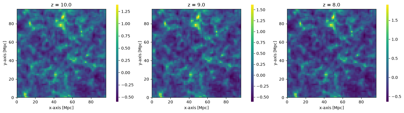
Any 3D field can be plotted, by setting the kind argument. For example, we could alternatively have plotted the dark matter density cubes perturbed to each redshift:

fig, ax = plt.subplots(1, 3, figsize=(14, 4))
for i, coeval in enumerate(coevals):
    plotting.coeval_sliceplot(coeval, kind="density", ax=ax[i], fig=fig)
    plt.title(f"z = {coeval.redshift}")
plt.tight_layout()

To see more options for the plotting routines, see the API Documentation.

This brief example covers most of the basic usage of 21cmFAST (at least with Coeval objects – there are also Lightcone objects for which there is a separate tutorial).

For the rest of the tutorial, we’ll cover a more advanced usage, in which each step of the calculation is done independently.

Advanced Step-by-Step Usage

Most users most of the time will want to use the high-level run_coeval function from the previous section. However, there are several independent steps when computing the brightness temperature field, and these can be performed one-by-one, adding any other effects between them if desired. In this section, we’ll go through in more detail how to use the lower-level methods.

Each step is performed by running a function which will return a single object. Every major function returns an object of the same fundamental class (an OutputStruct) which has methods to share its underlying data with the backend C code, and maintain knowledge of the state of its memory.

As we move through each step, we’ll outline some extra details, hints and tips about using these inputs and outputs.

The first thing to do is to set up the input parameters. Here, we’ll use the same basic set of parameters as we used in run_coeval, but with a different random seed, which ensures that we compute all new boxes.

new_inputs = inputs.clone(random_seed=42)

Initial Conditions

The first step is to get the initial conditions, which defines the cosmological density field before any redshift evolution is applied.

initial_conditions = p21c.compute_initial_conditions(
    inputs=new_inputs, cache=cache, write=True
)

As we said, all of these “single field” functions return objects of type OutputStruct. These objects have a few things in common. For example, they hold a reference to their input parameters:

initial_conditions.inputs.simulation_options.HII_DIM

64

More importantly, once computed, they hold the simulated data. Reading a field off the object gives you a plain numpy array. The Array objects that manage that data – tracking whether it is in memory, on disk, or shared with the C backend – live alongside it, under the .arrays attribute:

initial_conditions.arrays.keys()

dict_keys(['lowres_density', 'lowres_vx', 'lowres_vy', 'lowres_vz', 'hires_density', 'lowres_vx_2LPT', 'lowres_vy_2LPT', 'lowres_vz_2LPT', 'hires_vx_2LPT', 'hires_vy_2LPT', 'hires_vz_2LPT'])

Getting the underlying data

Reading a field attribute gives you a numpy array, and you can use it exactly as you would any other:

initial_conditions.lowres_density.mean()

This works whether or not the data is currently in memory. 21cmFAST will often purge array data from memory to keep memory usage down – for example, automatically while iterating through the redshifts of a lightcone. As long as the data was written to disk (which happens by default when you pass write=True), reading the field simply loads it back for you.

The memory management itself lives on the Array, which you reach through .arrays. That is where you look if you want to know where the data currently is:

initial_conditions.arrays["lowres_density"].state

If we now purge the object, the data is dropped from memory, but stays on disk (because we passed write=True when computing it):

initial_conditions.purge()
initial_conditions.arrays["lowres_density"].state

Reading the field still just works – it is loaded back from disk on access:

initial_conditions.lowres_density.mean()

initial_conditions.arrays["lowres_density"].state

There is also an explicit .get(), which does exactly the same thing. It is handy when the field name is held in a variable:

initial_conditions.get("lowres_density").mean()

The memory tradeoff

As you saw above, reading a purged field caches the data back into memory. So simply inspecting one – even something as innocuous as .mean() in a notebook cell or a debugger – will quietly reallocate that memory. This is usually what you want (you probably want the data close by if you are about to use it more than once), but it can be a surprise in a long-running script that purges aggressively to stay within a memory budget.

Two things make this traceable. Merely looking at the object (repr(), hasattr(), and so on) never triggers a disk read – only actually using the data does. And every read from disk is logged at DEBUG level, so if you are chasing unexpected memory growth or repeated disk traffic, turn on debug logging for py21cmfast and you will see exactly which arrays are loaded, and how often.

If you do not want the caching, disable it with the ``CACHE_ARRAYS_ON_ACCESS`` config option, either globally or (better) for a specific block of code via the config context manager. With it disabled, reading a purged field still re-reads it from disk each time, but nothing is retained afterwards. Note that this affects only this implicit path: .get() always caches, regardless of the setting.

initial_conditions.purge()

with p21c.config.use(CACHE_ARRAYS_ON_ACCESS=False):
    print(initial_conditions.lowres_density.mean())
    print(initial_conditions.arrays["lowres_density"].state)

A few practical tips for managing this:

• If you are inspecting a purged array just once and do not want to hold on to it, either wrap the inspection in config.use(CACHE_ARRAYS_ON_ACCESS=False), or simply call .purge() again afterwards to release it.

• If you are going to use a value repeatedly, let it cache (the default) – that avoids re-reading the same data from disk on every access.

• Use .has("field_name") to ask whether a field has data available at all (in memory or on disk) without loading it. A field that exists but has never been computed raises when you read it, rather than handing you None.

• Reach for output_struct.arrays["field_name"] when you want the Array itself – its state, its cache backend, or the functional transitions between them.

initial_conditions.load_all()
initial_conditions.has("lowres_density"), initial_conditions.has("lowres_vcb")

{note} Before v4.3 these field attributes gave you the `Array` object rather than the data, so you had to reach for `.get()` or `.value` to get a numpy array out. They now return the array itself. For one release the returned array still answers the old `Array`-only attributes (`.value`, `.state`, ...) with a deprecation warning, so existing code keeps working -- but they will be removed in v5.

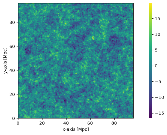
The coeval_sliceplot function also works on OutputStruct objects (as well as the Coeval object as we’ve already seen). It takes the object, and a specific field name. By default, the field it plots is the first field in arrays (for any OutputStruct).

plotting.coeval_sliceplot(initial_conditions, "hires_density");

Perturbed Field

After obtaining the initial conditions, we need to perturb the field to a given redshift (i.e. the redshift we care about). This step clearly requires the results of the previous step, which we can easily just pass in. Let’s do that:

perturbed_field = p21c.perturb_field(
    redshift=8.0, initial_conditions=initial_conditions
)

Note that we didn’t need to pass in any input parameters, because they are all contained in the initial_conditions object itself. The random seed is also taken from this object.

Again, the output is an OutputStruct, so we can view its fields:

perturbed_field.arrays.keys()

dict_keys(['density', 'velocity_z'])

This time, it has only density and velocity (the velocity direction is chosen without loss of generality). Let’s view the perturbed density field:

plotting.coeval_sliceplot(perturbed_field, "density");

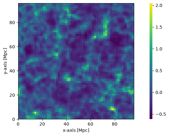
It is clear here that the density used is the low-res density, but the overall structure of the field looks very similar.

Ionization Field

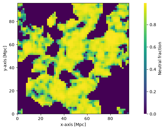
Next, we need to ionize the box. This is where things get a little more tricky. In the simplest case we are using in this tutorial, the ionization occurs at the saturated limit, which means we can safely ignore the contribution of the spin temperature fluctuations. This means we can directly calculate the ionization on the density/velocity fields that we already have.

ionized_field = p21c.compute_ionization_field(
    initial_conditions=initial_conditions, perturbed_field=perturbed_field
)

Let’s see the fieldnames:

ionized_field.arrays.keys()

dict_keys(['neutral_fraction', 'ionisation_rate_G12', 'z_reion', 'mean_free_path', 'kinetic_temperature', 'unnormalised_nion'])

Let’s plot the neutral fraction:

plotting.coeval_sliceplot(ionized_field, "neutral_fraction");

Brightness Temperature

Now we can use what we have to get the brightness temperature:

brightness_temp = p21c.brightness_temperature(
    ionized_box=ionized_field, perturbed_field=perturbed_field
)

This has only a single field, brightness_temp:

plotting.coeval_sliceplot(brightness_temp);